We all know more or less what Google Sheets provides to make life easier for its users. You can always get a workaround, no matter how big and complex your Google data sheets are. And to find that workaround, you don’t need to be a tech expert. Simply put, it doesn’t matter at all whether you’re a newbie to Google Sheets or a pro. So, to become a pro in Google Sheets, you need to be a master of Google Sheets functions.
In this article, I’ll be with you, covering 10 essentials Google Sheets functions by which you get rid of hours of workload. It’s time to make your work life easier by knowing essential Google Sheets functions.
Essential Google Sheets Functions
Before heading toward the advanced hacks of Google Sheets, you need to know some essential functions and formulas at first. Once you realize these basic functions, you won’t be stuck with any datasheet.
In fact, you’ll understand which formula or functions you need to apply to get a workaround for any complex situations. Well, let’s dive into the functions one by one with the proper examples below.
1. SUM Function: Use to Add Multiple Numbers
Adding numbers is the easiest but most important primary Google Sheets function. With the SUM function, you can easily add considerable numbers, add numbers of multiple cells, and use numbers as a combination.
The syntax of the SUM function is SUM(value1, value2, vlaue3,….). The value1 is a must requirement, and other values are optional for working with this function.
For example, if you want to add numbers 25, 30, and 25, you need to apply the below formula.
=SUM(25,30,25)
Or, if you want to add numbers of cell A1 to A5 based on the below example sheet, then your formula will be this-
=SUM(A1:A5)

2. COUNT Function: Use to Count Google Sheets Cells with Numbers
What if you want to count multiple cells and figure out how many cells have numbers? In a situation like this, the COUNT function comes into play.
And the syntax of this function of Google Sheets is COUNT(value1, value2,….). Here also, value1 is a must requirement, and other values are optional.
To count cells from A1 to A6, you need to use the below formula to get the number of cells that contains numbers.
=COUNT(A1:A6)

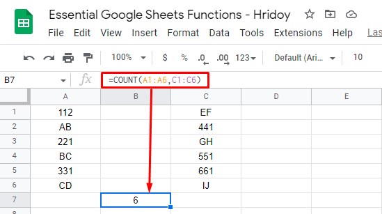
Another example could be the below one. To count A1 to A6 and C1 to C6, you have to use the below formula now.
=COUNT(A1:A6,C1:C6)

As you can see from the result, a total of 6 cells contain numbers in the above datasheet.
3. AVERAGE Function: Use to Calculate Numbers Average
There are many situations when you will be in need to find out the average of multiple numbers or multiple numbers in a range of cells. Well, the syntax of the AVERAGE function is Google Sheets is AVERAGE(value1, value2,…).
Let’s figure out what is the average of 20, 30, and 40 by using the average formula below.
=AVERAGE(20,30,40)

If you wish to figure out the average number of cells A1 to A5, you need to apply the below formula now.
=AVERAGE(A1:A6)

4. CLEAN Function: Use for Removing Non-printable Characters
The CLEAN the function is another useful function in Google Sheets. You can use this function to remove non-printable characters such as returns and backspaces.
However, when you import and insert something in Google Sheets from other sources, there might be a possibility of having non-printable characters (visible or non-visible) there.
Using this function, you can remove these characters easily. This is the syntax of the CLEAN function CLEAN(text); without any text, the function will now work.
For example, you can remove the non-printable characters from cell A1 (below sheets) by applying this formula.
=CLEAN(A1)
N.B: Since the function removes both visible and non-visible characters, some cases may not notice any differences whatsoever in the resulting cell.
5. NOW and TODAY Function: Use to Find Current Date and Time
To see the current date and time whenever you open your Google Sheets, you can apply the NOW and TODAY functions. The NOW is the function that displays the date along with the time, whereas you only get the current date with the TODAY function.
Here is the syntax of these two functions- NOW(), TODAY(). Interestingly, you don’t have any arguments for these formulas. You need to type these syntaxes in any cell on your Google Sheets to get the result. See the examples below-

Moreover, if you prefer to get the date and time in any specific format, you can also ser that in your Google Sheets.

6. TRIM Function: Use to Remove White Space
To tide up your sheet (removing white spaces between the texts), you can use the TRIM function in your Google Sheets. It works just like Microsoft Excel.
Either the text can be any cell references or any text itself. Here is the syntax of this formula TRIM(TEXT).
For instance, you can use the formula below to remove the white space from cell A1 texts.
=TRIM(A1)

Also, if you wish to remove white space from “Use To Remove White Space,” you can use the below function.
=TRIM("Use To Remove White Space")
7. IMAGE Function: Use for Inserting Image in Cells
As we all know, Google Sheets has the feature for inserting images into cells. On top of this, you can use the IMAGE function, an extra feature, to resize, setting up height and width in pixels as you want.
The syntax of this function: IMAGE(url, mode, height, width). Having the URL is a must in this function, whereas other arguments are not compulsory.
If you want to insert an image using a URL, follow the below formula.
=IMAGE("https://ubuntupit.com/wp-content/uploads/2020/06/YouTube-DL-on-Linux.jpg")
Or, if you wish to insert images with custom height and width, below one is the formula then.
=IMAGE("https://ubuntupit.com/wp-content/uploads/2020/06/YouTube-DL-on-Linux.jpg",4, 50, 200)
In the formula, the number 4 indicates the syntax mode of the function, allowing the image size of 50 by 200 pixels.
8. CONCATENATE and CONCAT Function: Use to Combine Values or Texts
There are no perfect functions in Google Sheets more than CONCAT and CONCATENATE to combine things up. The items can be text, values, or even strings. Between these two functions, CONCATENATE offers more flexibility. It can merge words or values and insert spaces in between.
The syntaxes CONCATENATE(string1, string2,….) and CONCAT(value1, value2,….). Except for string2, all the arguments are mandatory to work these functions.
If you want to merge values of cells A1 and B1 in the below sheet using CONCATENATE, use the following formula-
=CONCATENATE(A1, B1)

Plus, if you wish to combine values 12 and 7 using CONCAT, the below formula will work-
=CONCAT(12,7)

Lastly, if you want to combine the texts of cells A1, B1, and C1, use the following formula-
=CONCATENATE(A1," ",B1," ",C1)

9. ISEMAIL and ISURL: Use to Validate Link or Mail Address
If you want to check the validity of things you’re inserting or importing in your Google Sheets, you can use ISEMAIL and ISURL Google Sheets functions.
Using ISEMAIL, you can have an email address validity, whereas, to check the validity of a URL, use ISURL.
The syntaxes are for these formulas ISURL(value) and ISEMAIL(value). Cell references and texts both work in these functions.
The results you’ll get as: TRUE and FALSE. If valid, that will result as TRUE; if non-valid, then the only option you’ve.
For example, in the below sheet, there are two mail addresses (in cells A1 and A2). Once is valid and another is not. To get the following result, you need to use the below formula-
=ISEMAIL(A1)
=ISEMAIL(A2)

Now, to check a URLs validity in cell A1, use the below formula-
=ISEMAIL(A1)

Finally, to check the URL of cell A1, you can use the following formula-
=ISURL("www.bytesbuzz.com")
10. SPLIT Function: Use to Separate Texts
SPLIT the function is the total opposite of CONCATENATE the function in Google Sheets. You can merge texts, values, and strings using CONCATENATE, whereas SPLIT functions work to separate texts, values, and strings.
Let’s see the below example. Here you can separate each word of cell A1 into three different cells. To do so, the formula will be-
=SPLIT(A1, " ",)

To know even more about Google Sheets functions, you may look at the usage of AND and OR functions or how you can hide errors in Google Sheets using the IFERROR function.
Wrapping Up
Well, that was all for now. Using the Google Sheets functions makes your work more effortless than ever before. Moreover, these functions can reduce your workload and help you get a workaround for any frustrating situations with Google datasheets.
It doesn’t matter whether you’re a newbie or an expert on Google Sheets formulas. However, the 10 Google functions mentioned above will be helpful for you. Your need to know and practice the usages of these functions daily.
I hope you liked it. Please share the post with others to let them know and leave your valuable comment in the below comment box. Be with UbuntuPIT; I’ll be back with other Google Sheets hacks- basic to advance level.


