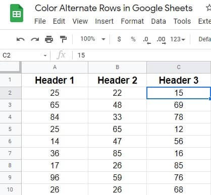
Let’s assume you have a Google sheets with an abundance of data and formulas. And it’s very obvious that you might feel bored and frustrated to operate these kinds of sheets. That is why many people tend to color alternate rows in Google sheets. By doing so, you can give your eyes a treat from monotonous data work and make your work easy and fast.
To the entire post, you’ll walk through how you can easily apply alternate shading to rows. However, I’ll show you the build-in process along with the conditional method if you wish to color every 3rd/4th/5th row.
Color Alternate Rows in Google Sheets
Google sheets are constantly updating its features. And coloring every other row using the built-in method is one of them to make your sheets more readable than ever.
However, it’s very old-fashioned nowadays to use conditional formatting to color alternate rows. But no worries! Now you can get this done with some easy clicks.
Well, let’s get to the business then, and get familiar with the process of coloring the alternate rows in your Google sheets.
1. Color Alternate Rows using Google Sheets Built-in Method
Let’s take a look at some easy steps below to color alternate rows using the Google sheets built-in method first.
i. At first, prepare or choose your datasheet on which you wish to have color alternate rows. Here’s an example:

ii. Look at the top menu bar, and find Format. Click to get further instructions accordingly.
iii. The below-resulting page will appear once you click on Format. Now scroll to the down and tap on Alternating colors.
iv. Here you’re on the page you’re looking for. Set all the styles and color options whichever you wish to have in your sheets. However, make sure the Header and Footer have blue tick if you’ve any. Well, after seeing all things up, click Done.
v. Here’s the final result after using the built-in Google sheets method. Now you can see, every other row has a different color which you’ve chosen a minute before.
2. Color Alternate Rows using Custom Formula
Along with the built-in method, Google sheets have custom formulas to color alternate rows. And to show you the process, I’m using the same datasheet which I’ve shown to you in time of the built-in method. Let’s start with the process:
i. Obviously, select all the data on which you would like to apply formulas to color alternate rows in Google sheets. However, before going further, make sure you select those cells that consist of data. I mean, select all the cells except the Header and Footer if you’ve in your sheets.
ii. Find the Format option from the top menu bar. Click on it and select Conditional formatting from the popped-up result.
iii. You’ll find the below-resulting page now. Find the Format rules section and tap to get the dropdown values. And finally, to apply formulas select Custom formula is option here.
iv. Well, now it’s time to set the formula and formatting style. Here’s the formula =ISEVEN(ROW()) you need to put IT under the Custom formula is section.
v. Well, the process completes here. The below-resulting page is the final look after applying the formula of coloring alternate rows in Google sheets.
3. Color Every 3rd/4th/5th Rows Using Custom Formula
So far, I’ve discussed coloring alternate rows in Google sheets. But, what if you would like to color every 3rd, 4th, 5th row in your Google sheets, then how to do that? You just need to apply a simple formula to get things done. Let’s start with the steps:
i. Imagine the same datasheet in procedure also. Like before, select All cells of the sheets>Format>Conditional formatting to reach the below-resulting page where you need to choose Custom formula is.
ii. Well, it’s time to write the formula up. In my case, I’m coloring every 3rd row of the sheets. Here’s the formula for doing this: =MOD(ROW(),3)=0
If you wish to color 4th/5th and any other rows then just replace 3 with the number 4/5 in the formula. However, choose your formatting style with color and click on Done.
iii. Here’s the result of every 3rd row after using the custom formula. In my case, I included the Header section in the formula as well. That’s why the result is appearing like this.
Wrapping Up
Well, it’s time to wrap things up. I think you know from now, how to color alternate rows in Google sheets. However, clarity and readability are the key factors whenever you work with numbers and texts.
Luckily, Google sheets are providing you with the feature of doing so through built-in methods as well as the functional process. However, feel free to share the process with your closed ones and leave a comment in the comment section below.
Well, taking leave now, and I’ll be back shortly with any other Google hack. Till then, take care and always keep yourself updated with UbuntuPIT’s latest tips and tricks.