When we work in Google Sheets, you may require absolute values of any numbers. However, absolute means the distance between a number and zero. It will always be a positive number. For instance, 10 is the absolute value of 10, and -10. So, if you want to know how to find absolute value in Google Sheets, you’re certainly in the right post.
However, it can be very useful to know how to find absolute values for various purposes. And there are several processes available for finding the absolute values in Google Sheets. In this article, I’ll walk you through 4 different ways of finding absolute value in Google Sheets.
Find Absolute Value in Google Sheets
If you have a negative sign in your numbers, an absolute value is all about removing the sign from that number. Assume you have a large numerical dataset and want to have all the values as absolutes. Therefore, removing the negative sign from each number manually would be time-consuming and not a good idea.
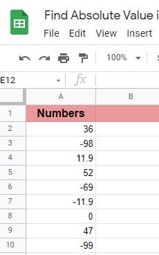
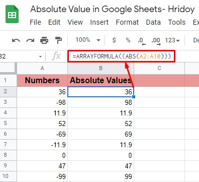
I’ll use the following dataset below to demonstrate all the procedures. As you can see, both negative and positive values are present in the dataset. Let’s begin without saying any more.
Method 1: Convert All Negative Numbers to Positive
The method title says all. Just convert all negative numbers to positive, and you’ll find the absolute values eventually. Though there are several ways available to get this done, IF the function would be the easiest one.
Once you apply the IF function to any negative numbers, it’ll check whether the number is less than 0 or not. And, if it is, multiply the number with -1. As a result, you can find absolute value in Google Sheets for each negative number.
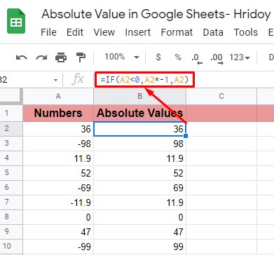
Here’s the function below by which you can convert all the negative numbers to positive ones. Type or paste the below function in cell B2 and apply autofill to have values in the rest of the cells.
=IF(A2<0,A2*-1,A2)
Method 2: Use Google Sheets ABS Function
To find the absolute value in Google Sheets, using the ABS function could be another easy way. The syntax of the function is below-
ABS(value)
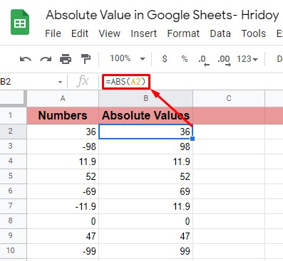
The value in the syntax refers to the number for which you wish to find the absolute value. Now apply the formula below by typing or pasting it to cell B2 in the above example datasheet.
=ABS(A2)
Boom! See the result below. And to get the absolute value for the rest of the numbers, either drag the B2 cell down from the right corner or use the auto-fill feature of Google Sheets.
Besides, another formula mentioned below helps you to find absolute value in Google Sheets in one go. No auto-fill, no dragging down is required here. Just paste or type the formula in cell B2 and see the result.
=ARRAYFORMULA(ABS(A2:A10))
Method 3: Use Google App Script to Find Absolute Value
Using Google Script or Apps Script would be another great way to find absolute value in Google Sheets. You need to apply the custom app script on the list of values you have to convert into absolute values.
You need to apply the app script below to find absolute value in Google Sheets.
function findAbsolute() {

var app=SpreadsheetApp;

var ss=app.getActiveSpreadsheet();

var activeSheet=ss.getActiveSheet();

var range=activeSheet.getActiveRange();

var values=range.getValues();

var value;

for (var i in values){

var row=values[i]

for (var j in row) {

value=row[j]

if (value<0){

row_num=parseInt(i)+1;

col_num=parseInt(j)+1;

console.log(value)

console.log(row_num, col_num)

activeSheet.getRange(row_num+1,col_num).setValue(value*(-1));

}

}

}

}
Now, let’s see the step-by-step procedure of applying the app script to your Google Sheets.
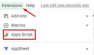
Step 1: In the first place, go to your Google Sheets on which you would like to apply the above Apps Script. Once you’re in, hover over Extensions from the top and choose Apps Script.
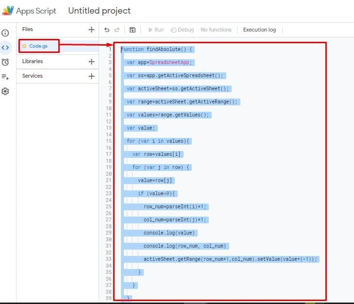
Step 2: The last step redirects you to the below-resulting page. The apps script window is now open for you. Copy the above code and paste it here to replace the existing demo one. You can rename the script from Untitled to FindAbsolute so that you can import the code into your Sheets easily.
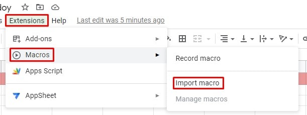
Step 3: Now, go back to your Sheets where you’ve all the values from which you wish to find the absolute ones. Again hover Extensions and then Macros>Import macro to import the Apps Script code into your Sheets.
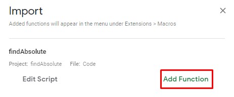
Step 4: In this step, you can see the below page that contains the Apps Script. According to my last instruction, you can easily get the script here if you’ve renamed it. In my case, I renamed the script as findAbsolte. So find yours and click on Add Function.
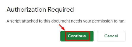
Step 5: If you’re trying to apply Apps Script for the first time in your Google Sheets, you’ll get the below-resulting page. It’ll ask for your Email authorization. So, click on Continue to set all things up regarding the authorization process.
Once everything is complete, your Apps Script runs automatically into your Google Sheets, and you’ll find the absolute value you wished for.
N.B: There’s a feature available by which you can run the scripts and convert the values easily. That is, add a button to your sheet and link it with your preferred script. By doing so, you could select and convert a range of cells to their absolute value with a simple click on the button.
Method 4: Using Add-on
To find the absolute value in Google Sheets, using an add-on is another way. It eventually converts the negative numbers to positive ones and provides you the absolute value.
Power Tool is the add-on you need to get going with the process. So, if you don’t have the add-on installed in your Google Sheets, please install it first.
Install Power Tools Add-on: To get and install the add-on, go to your Google Sheets, hover over the top menu, and click on Extensions. After that, choose and click Add-ons>Get add-ons.
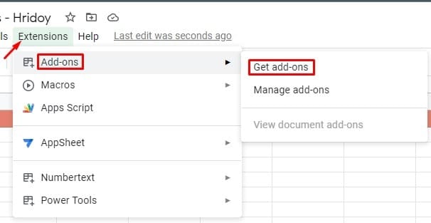
Right now, you’re in the Google Workspace Marketplace. You’ll get all the add-ons here, and to get the Power Tools, go to the search box and type.
However, by typing just Pow, the Power Tools add-on will be visible to you in the search result. Select the add-on and install it accordingly into your Google Sheets.

Run the Add-on and Find Absolute Value: Once you install the add-on in your Google Sheets, go back to the sheet. And follow the below procedure step-by-step.
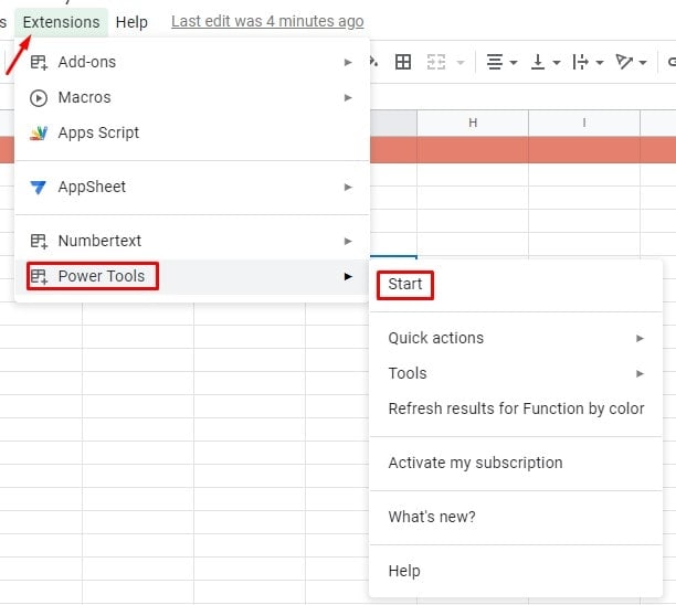
Step 1: Again, move your cursor over Extensions from the top, and you’ll get the add-on list you’ve installed so far in your Google Sheets. As you can see, Numbertext and Power Tools are the add-ons that, so far I’ve installed.
However, now select Power Tools from the resulting page and click on Start further to run the add-on in your Google Sheets.
N.B: If you can’t see the add-on you just installed, close the file and re-enter it. If this will not work too, restarting your device is the only option left.
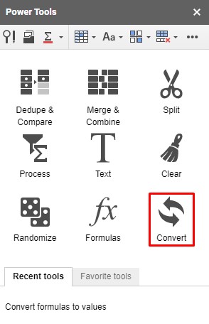
Step 2: At this point, you’ll be seeing the below-resulting page. Click on Convert from here.
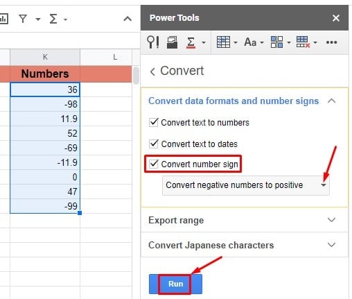
Step 3: Here you come to the last step. Select the range of numbers and go to Power Tools’s Convert section that you opened a few moments ago.
Now, check the Convert number sign box first. Ensure the Convert negative numbers to positive is selected in the dropdown under the Convert number sign.
Now hit the Run from the bottom since all checking and selecting is complete. And see the magic in your selected range of numbers. You’ll notice all your negative numbers turned into positive ones.
Wrapping Up
It’s a wrap of procedures to find absolute value in Google Sheets. 4 methods have been explained above; you can with whichever you find easy. The first two methods are all about applying formulas, whereas the last two can be tricky if you’re new to Google Sheets. However, each method has its individuality. So, go with the one you prefer the most.
If you find this post helpful and worth sharing, share it with others and comment about your experience with it in the comment section below. I’ll be back to the business soon with another Google Sheets trick.
