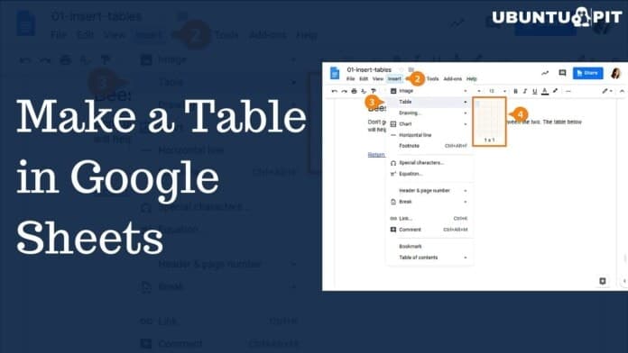
Unfortunately, Google Sheets doesn’t offer any method of inserting a table directly. But, no worries! You can make a table in Google Sheets in other ways.
The first could be that you can make anything using filters and borders that will be looking like a table. And the best possible workaround to make a table in Google Sheets would be using a table chart.
As we all know, Google Sheets is a tool for data but tables can add extra benefits to it. For example, shorting the data within the table is possible while keeping the non-table data untouched in the sheet.
Also, you can color alternate rows and other different styles to provide your table easy viewing experience.
Making a Table in Google Sheets Using Table Chart
Please note that having a large amount of data and manipulating them in Google Sheets will not be easy to do with a table chart.
In a scenario like this, you need to use Google Sheets’ pivot table. On the other hand, if you don’t need any extensive tools, then going with a table chart will be a great option.
Here’s the step-by-step procedure below to make a table in Goole Sheets using a table chart.
1. Start with visiting Google Sheets, sign in to your account and then open the sheet that has the data.
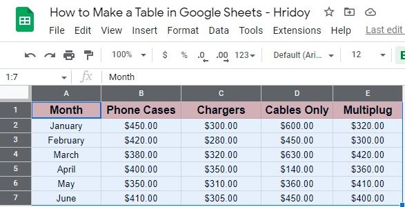
Now, simply select the data (on which you want to have the table) by dragging your mouse cursor through the cell.
What if you may add more data to the sheets? No worries, you can adjust the cell range later on when you wish.
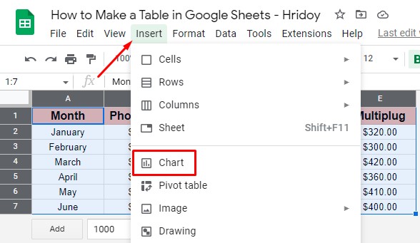
2. Now hover your cursor over the top menu bar and click on Insert, and select Chart from the resulting menu.
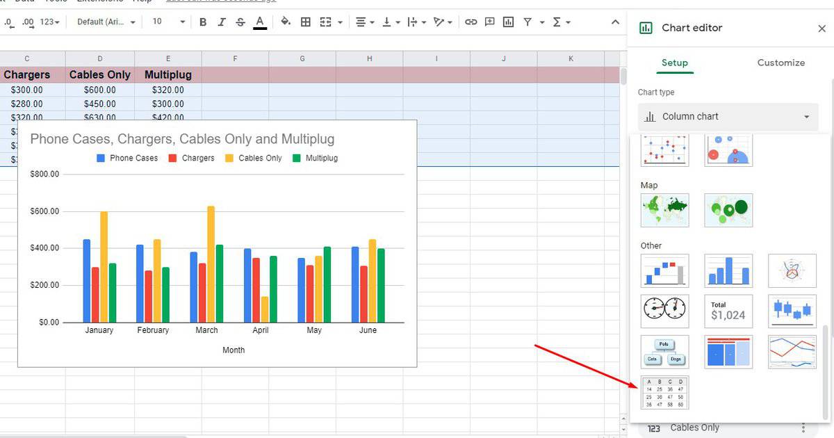
3. Once you click on Chart, Google Sheets provide you a chart type by default with a Chart Editor sidebar at the right on your sheet.
However, as you wish to have a Table Chart, so go to the sidebar and click on the Chart type dropdown.
And you’ll get plenty of pre-installed chart types there. Now scroll down to the bottom, and you’ll find a Table Chart under the Other category. Click on it.
4. This brings you a new table type automatically. Well, now you can adjust the as you want along with the way of displaying your table from the Chart Editor sidebar.

Setting Up the Table in Google Sheets
Well, as you’ve already put your table in your Google Sheets, it’s time to set up the table. However, you can set or modify the table from the Chart Edit sidebar whenever you want. You’ll get all the options there to set your table up. Here’s explained below how you can set up the table-
You can reopen the Chart Edit sidebar if you ever closed it. To do so, you need to select the table chart by clicking on it, and you’ll notice a three dots icon on the top right corner of it. Well, now select the Edit chart from there.
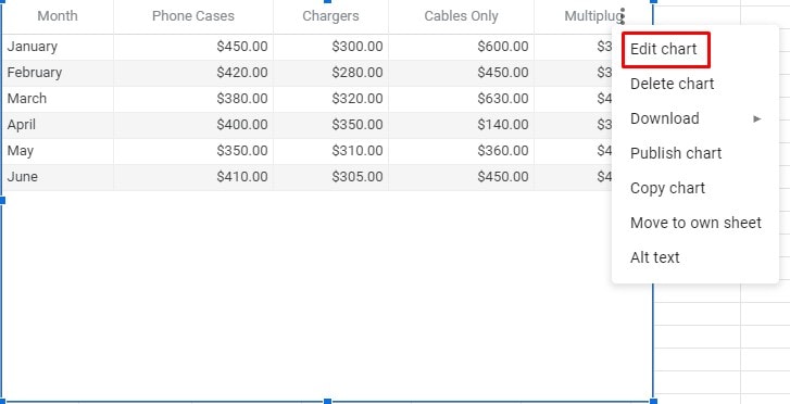
Here you are in the main section. In the right sidebar, you’ll see a section named Setup. Click on it to work further with your data table chart in Google Sheets.
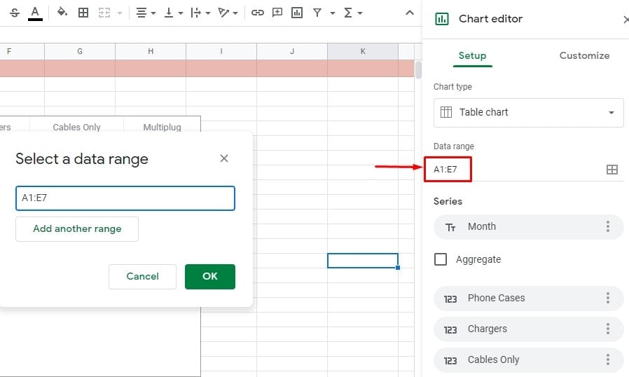
You’ll see several options there- Data range, Series, Add More Series. And can adjust these sections as you want.
Let’s see what these sections are and how you can set these up properly.
Data Range of Your Table Chart
This section refers to the data range of your table. So, confirm your data range here. Besides, you can add or minus the data range.
And to add another range, you need to click on the right side. Either you can choose ‘Add Another Range‘ or use any of the default suggestions.
Series Section of Your Table Chart
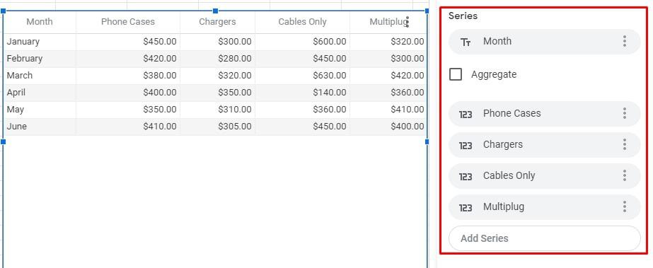
You’ll get different series options here. It mainly refers to how you want to display your data.
However, as you can see, a first series is already selected there, but you can change and select a different one as your first series.
This indicates the data that you have a far-left column of your table in Google Sheets. Additionally, to Aggregate the data, you can check the box here.
Moreover, you can change, add, or remove any of the different series for the columns of data. And, if you wish to include another series, click on the Add series section below and select the cells.
More Options for Your Table Chart
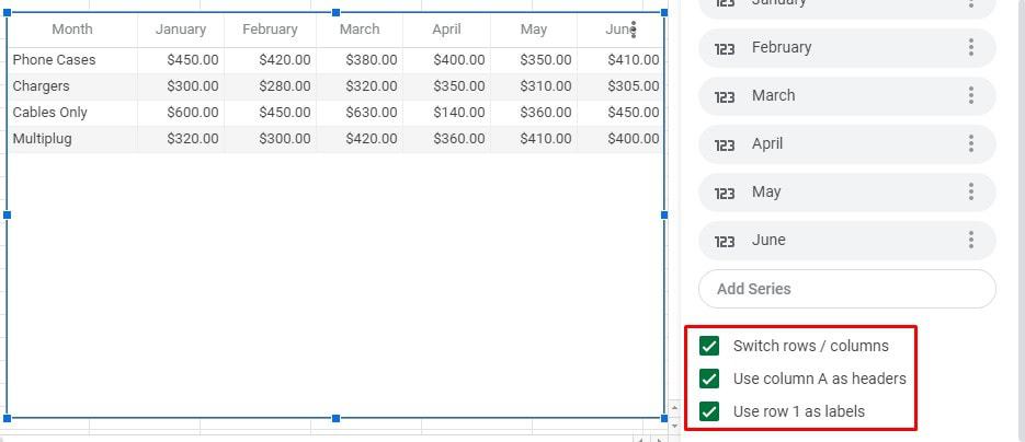
At the bottom of the Setup section, you’ll get extra check box options to set up your table. Through the checkboxes, you can switch rows/columns, use column A as headers, and use row 1 as labels. Set up your table chart by using these extra options depending on your preferences.
Customizing the Table Chart
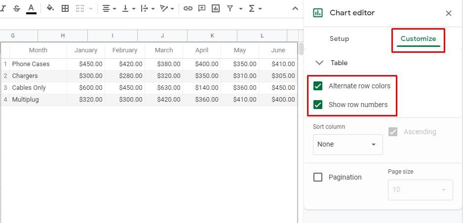
Once you set up your table data the way wished for, now you can customize your table chart’s appearance. To do so, you need to go to the Chart Editor sidebar from the right and choose to Customize section from there.
This allows you to customize a collection of options (rows and numbers, sorting, and pagination). Let’s click on Table to expand.
Customize Rows and Numbers
If you wish to alternate the colors and want to display the row numbers, check the boxes below the Table section.
Column Sorting
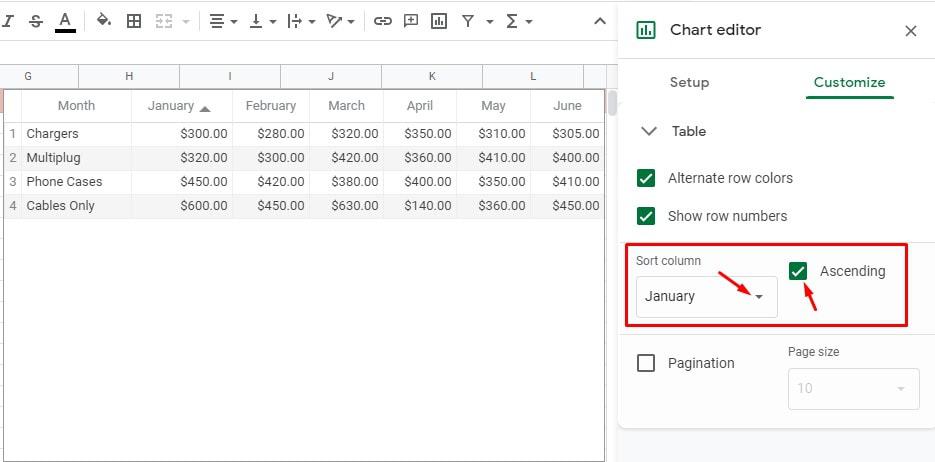
To use a default column for sorting the data, you need to select it from the drop-down list. Plus, if you wish to set the data in Ascending order, then check the box on the right side.
What if you don’t select a default column to sort? No worries, you’re open to sorting your data by any column.
And to do this, you need to select the column header by which you want to sort the data. Your data table updates automatically.
Pagination
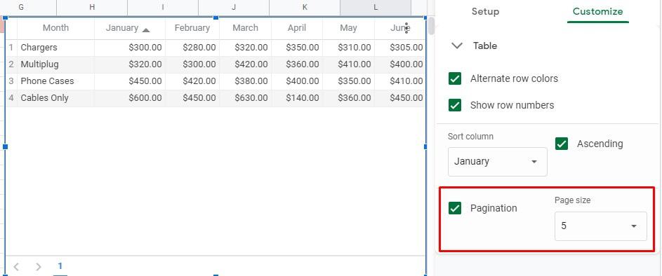
You may have a massive amount of data in your Google Sheets table. Here comes the, pagination comes into the play. You can select your page size (5 to 100) from the below-marked dropdown section.
And you’ll see the results at the bottom of your page. It adds both arrows and page numbers. Using arrows and page numbers, you can see all the data tables that have been classified into different pages.
Though the table is not that popular in Google Sheets, still, you can make it like other famous Google Sheets charts. You can place your table chart anywhere on your sheets once you complete it.
Besides, you can also resize your table by dragging in or out and also corner to edge. The most amazing part is its automation. Whenever you update cell range data, your table chart updates automatically.
Closing Statement
It’s a wrap. From now on, you can make a table in Google Sheets if your wish to. You may have used Microsoft Excel always to make a table; let’s try something new. There is no direct option for making a table in Google Sheets like Microsoft Excel.
But, you can create a similar table with the same functionalities. Moreover, you can customize several other things to your table in Google Sheets.
So, to improve your productivity, you can also use the Google Sheets table feature. I hope you liked the post. Let me know your feedback on it.
Plus, share the post if you find it helpful and worth sharing. I’ll be back soon, along with another Google Workspace hack. Till then, take care and always keep yourself updated with UbuntuPIT.
