Undoubtedly, Google Sheets’ QUERY function is one of the most influential and versatile functions. Whether your query or problems are- simple or complex, you can get a workaround through the QUERY function. However, if you’re a newbie to Google Sheets functions, it may seem not very easy to you. But once you understand the primary usage of the QUERY functions, you’ll undoubtedly enjoy it. So, the post is all about the different usage of the QUERY function in Google Sheets.
I’ll be with you in the entire post to let you know what precisely the QUERY function is, its syntax, and its different usage? There are tons of scenarios where you can apply the QUERY function, but I’m going to show you some prominent ones. If you can cover the below usages of this function, you can surely understand its whole.
QUERY Function in Google Sheets
If you want to play with your Google Sheets datasheet, the QUERY function is the only player. You can manipulate your datasheet with logic. You can even do filters, find averages, and do sums with it in your Google Sheets. So, once you get the sense of it, you can do many things with your datasheet.
Understanding the QUERY function will be super easy for you if you’re familiar with SQL. The format of SQL and QUERY is more or less the same. So, if you already know about SQL searches, QUERY will be a piece of the cake. If not, no worries! I’m here to help out with suitable examples.
Before diving into the real business, let’s get familiar with the QUERY function format. This is the format of QUERY functions in Google Sheets: =QUERY(data, query, headers).
- Data- This will be the cell range of your datasheet. For inastance “A2:E12” OR “A:E“.
- QUERY- Depends on what your search query will be.
- Headers- It indicates the data range of your top cell.
Please note that you may have a header including two cells, and the QUERY specifies them combined as one header.
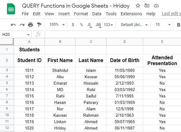
Demo Datasheet of the Student List
Here is a datasheet example below of a list of students. The sheet includes the students’ names, students’ IDs, date of birth, and whether they’ve attended the presentation or not.
1. Find Out the List of the Names Who Didn’t Attend the Presentation
You can use the QUERY function to find out the list of the names who didn’t attend the presentation and their IDs. To do so, you need to open a second sheet. On that sheet, you’ll pull all the data from this sheet to get your expected result.
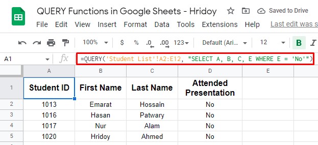
The formula you need to apply here is, =QUERY('Student List'!A2:E12, "SELECT A, B, C, E WHERE E = 'No'"). This formula will calculate the data from range A2 to E12 on the Student List sheet.
As you can see in the below result, you have got the list of those who didn’t attend the presentation in a separate sheet. However, along with the name, the QUERY function provided student IDs and the result you were looking for too.
2. Extend the Range of Data and Make the QUERY Function Automatic
The above QUERY function worked within a specific range of data, but you can make it more dynamic. What if you add some students’ names further to get results as well? Then the above formula won’t work.
What you can do is, change the query to all the data in columns A to E. If you do so, whenever you add any more student names to the sheet and look for whether they attended the presentation or not, your formula will also update automatically.
As a result, you’ll get your desired result without applying the procedure again and again.
To do this, you need to apply this QUERY formula now =QUERY('Student List'!A2:E, "Select A, B, C, E WHERE E = 'No'"). However, the formula won’t count initial cell A1(Students).
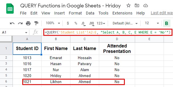
As you can see, ID 1021 (Likhon Ahmed) was not there in the initial demo datasheet. You’ve added the name later and applied the above formula.
From now on, if you add any more IDs, the formula will automatically calculate that. So, as the QUERY formula update, your results update automatically.
QUERY Formulas with Other Functions – Advanced
As I said, the QUERY function is the most versatile one. You can use this formula with many other logical operations. For example, you can use this formula with AND and OR functions or Google functions (e.g., COUNT).
However, not only with these, but you can also operate comparisons to find any result between two values, such as greater than, less than, and many more.
Usage of AND and OR Functions with QUERY
Perhaps, we all know about AND and OR: two nested logical operator functions. These two functions work well with the QUERY function. Using these combined, making multiple search criteria for the QUERY formula is possible.
1. QUERY with OR Function
A similar result is also possible when you use QUERY with the OR function. For example, you may want to search the student list born in the 1980s. You need to switch the dates and use OR function with your QUERY to get so.
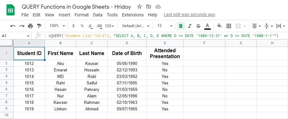
Now the formula will be this =QUERY('Student List'!A2:E12, "SELECT A, B, C, D, E WHERE D >= DATE '1989-12-31' or D <= DATE '1980-1-1'").
Here is the result. As you can see, this is the result of students born before or after the 1980s. So, it’s clear now that the remaining three students, out of ten in the demo datasheet, were born in the 1980s.
2. QUERY with AND Function
You can use AND to search the data between two dates of the demo datasheet. For example, you can sort all students’ born years. I’m going to dig out those students list who were born between 1980 to 1989.
However, you can also apply comparison operators greater than or equal to (>=) and less than or equal to (<=) in this formula so that it filters the datasheet as your instruction.
Here is the formula for this purpose =QUERY('Student List'!A2:E12, "SELECT A, B, C, D, E WHERE D >= DATE '1980-1-1' and D <= DATE '1989-12-31'").
The DATE function is also used in this formula that will calculate all birthdays of the students and find out the result between and equal to (01/01/1980- 12/31/1989).

As you can see, two students who meet the requirements were born between 1980 to 1989. So, you can use QUERY with AND and DATE functions to search between two dates.
Making Comparison Using QUERY
You can go with the QUERY function if you want to filter and narrow down the data. QUERY supports comparison operators (greater than, less than, or equal to), by which you can get your filtered results.
To show you, I’ve added an extra column (F) in the demo datasheet of the ‘Student List.’ The column contains the number of presentations each student attended.
Now, I’m using the QUERY function to find out the student list who attended at least one presentation. And to get this, the formula will be =QUERY('Student List'!A2:F12, "SELECT A, B, C, D, E, F WHERE F > 0").
In this formula, the greater than comparison operator (F>0) is to search values above zero in the F column.
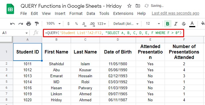
This is how you can make a comparison using the QUERY function. As you can see above, seven students attended at least one presentation, and the rest of the students did not participate in even one.
Usage of COUNT Function with QUERY
With the QUERY function, you can not only do simple searches to filter or narrow the data to get results, but you can also manipulate the data as you like.
And to do that, you need to mix the QUERY function with other Google Sheets functions. For example, the COUNT function.
Well, let’s see an example of this. Assume I want to get the number of how many students attended the presentation and how many are not at all by using the COUNT function with QUERY.
However, for doing as I said, the mixed function’s formula will be this =QUERY('Student List'!A2:E12, "SELECT E, COUNT(E) group by E").
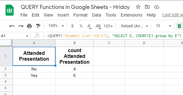
You can see that the results are above what you expected. In this example, the QUERY function focuses on column E (Attended Presentation), and the COUNT function counts the number of cases in which each type value (Yes or No) occurs.
And the result was accurate, six students attended the presentation, and four haven’t. However, for testing purposes, apply this formula in a short datasheet first to see whether this works accurately or not.
Final Verdict
Well, that’s how all things end here. If you went through the whole post, you could quickly get your query results using the QUERY function in Google Sheets. No matter how complex your query is, you can get the result out of that indeed.
Once you master the QUERY function, functions, and formulas in Google Sheets will be super easy for you. There are huge situations where you can apply QUERY functions, as I said before. And from them, some of the important ones are explained above.
However, I’m going to take a leave for now and hope that you’ll get benefits from the post. If so, share the post with your surroundings to let them know. And your thoughts on this will be appreciated. Therefore, leave a comment in the comment box below.
